SUM, IF, COUNTIF and XLOOKUP cover four common Excel tasks: totaling values, returning conditional results, counting matches and retrieving corresponding records. Reliable results still depend on correctly structured data, aligned ranges and a compatible Excel version.
The sequence starts with formula syntax and cell ranges before moving to a function for each task. A final check of the inputs, references and recipient's Excel version matters because a calculated value is not proof that the right cells were used.

Start with the formula and its cell range
Microsoft defines functions as predefined formulas that use arguments in a set order and says their structure begins with an equal sign, followed by a function name, parentheses and arguments. A direct calculation can look like =A1+B1, while a function-based formula can look like =SUM(A1:A2).
Microsoft's formula guide says formulas always start with an equal sign and shows that =SUM(A1:A2) adds the values in cells A1 and A2. In a reference, A1 identifies one cell, A1:A10 identifies a continuous range and A1:A10,C1:C10 passes two separate ranges.

Three decisions should be explicit before a formula is entered: which column supplies the data, which rows belong in the calculation and where the result should appear. Keeping one record per row and one type of information per column makes those boundaries easier to review.
Cell contents also need inspection before calculation. Microsoft says SUM ignores text in a referenced range and adds only the numeric values, while its COUNTIF guidance warns that leading spaces, trailing spaces and nonprinting characters can produce unexpected counts.

SUM makes the range visible
Microsoft documents SUM as a function that accepts individual values, cell references, ranges or a mixture of them, using the syntax SUM(number1,[number2],...). A total for order values in B2 through B10 is =SUM(B2:B10); two nonadjacent value columns can be combined with =SUM(B2:B10,D2:D10).

A range is easier to audit than a long chain such as =B2+B3+B4+B5. Microsoft's guidance says SUM ranges generally adjust when rows or columns are inserted or deleted within the reference, but a new row outside the referenced range can still be missed.
The result should be checked against a small manual sample and the visible boundaries of the range. Subtotal rows, headers or records from another reporting period can create a plausible but incorrect total if they are included.

IF converts one test into two possible results
Microsoft gives the IF syntax as IF(logical_test, value_if_true, [value_if_false]), returning one value when a condition is true and another when it is false. If C2 contains actual spending and B2 contains the budget, =IF(C2>B2,"Over budget","Within budget") labels the row after comparing the two values.
Text returned by a formula belongs inside quotation marks; an intentionally empty result is written as "". A status field can also be converted into a number with =IF(D2="Complete",1,0), allowing a later SUM formula to count the completed rows.

COUNTIF counts records that meet one condition
Microsoft defines COUNTIF as COUNTIF(range, criteria) and says it counts cells that meet one criterion. If A2 through A100 contain order statuses, =COUNTIF(A2:A100,"Paid") counts paid records; =COUNTIF(A2:A100,D1) instead reads the criterion from D1.

Criteria can be text, a number, a comparison such as ">1000" or a cell reference. Microsoft warns that stray spaces or nonprinting characters can stop apparently identical text from producing the expected count.
COUNTIFS is the related choice when every record must meet more than one condition. Microsoft says each additional COUNTIFS criteria range must have the same number of rows and columns as the first range, because the conditions are evaluated one row at a time.

XLOOKUP matches an identifier to a return value
Microsoft describes XLOOKUP as a search across one range that returns the corresponding item from another range, even when the return column is on the other side of the lookup column, and gives the syntax =XLOOKUP(lookup_value,lookup_array,return_array,[if_not_found],[match_mode],[search_mode]). The lookup and return ranges therefore need to describe the same rows.

Microsoft says XLOOKUP uses an exact match by default and returns #N/A when if_not_found is omitted. The formula =XLOOKUP(E2,A2:A100,C2:C100,"No match") supplies a readable alternative.
The alternative text identifies an absent match; it does not prove that the formula or data is otherwise correct. A misspelled identifier, an extra space or misaligned lookup and return ranges can still send the formula to the wrong outcome.

Choose the function from the task
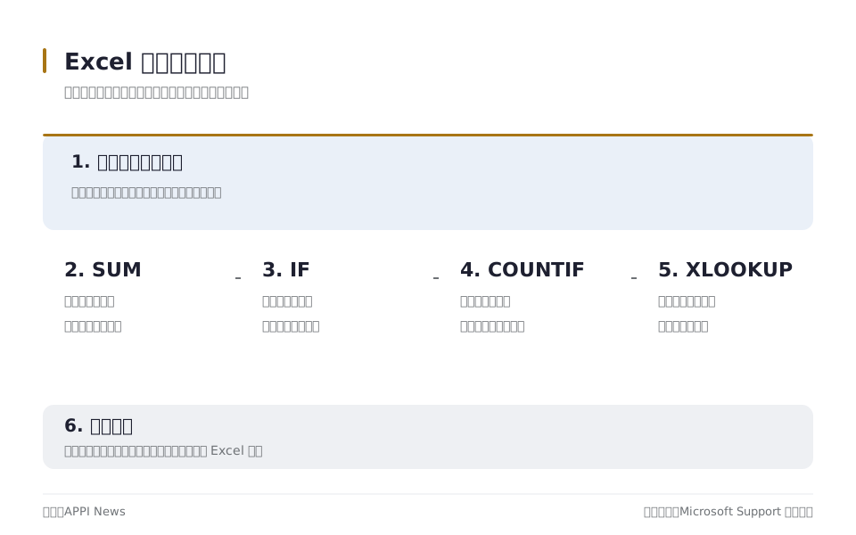
The four functions solve different problems, so the task should be described before the formula is selected. The input range and expected output provide a faster decision rule than memorizing syntax without a data example.
| Task | Start with | Check first |
|---|---|---|
| Total a set of amounts, hours or quantities | SUM | The range includes all intended records and no subtotal rows |
| Return one of two values after a test | IF | The logical test and both possible results are explicit |
| Count records that meet one condition | COUNTIF | The criterion matches the stored text or number format |
| Find a name, price or department from an identifier | XLOOKUP | The lookup and return ranges correspond row by row |
A displayed result still needs a formula check
A calculated number only shows that Excel evaluated the formula it received. The review should cover the function name, paired parentheses, every argument, the selected range, blank cells and the type of data stored in each source column.
Microsoft says a misspelled function name can return #NAME?, while a nested function that supplies an incompatible value to an argument can return #VALUE!. The error code narrows the search, but the underlying formula and source cells still need inspection.
Version compatibility belongs in the same review. Microsoft says XLOOKUP is unavailable in Excel 2016 and Excel 2019, although those editions can encounter the function in a workbook created with a newer Excel version.

How this plays out outside Taiwan
Microsoft sells Excel through country-specific consumer storefronts, so the route to the desktop app, the consumer license and the price displayed by Microsoft are market-specific. On September 9, 2026, Microsoft's United States store listed Microsoft 365 Personal, Family and Premium subscriptions alongside Office Home 2024. The United Kingdom store listed the same four purchase categories in pounds, while the Australian store displayed its offers in Australian dollars and the Singapore store displayed its offers in Singapore dollars. The pages demonstrate why a price from one market should not be treated as a universal quote; the relevant official store should be checked again at purchase.
The product rules matter as much as the amount. Microsoft describes Microsoft 365 Personal as a subscription for one person, Family as shareable with up to five additional people and Office 2024 as a one-time purchase for one computer. Its United States comparison page says each Family member can use the apps on up to five devices simultaneously, while specified artificial intelligence benefits remain with the subscription owner. The recipient's Excel app and version therefore remain part of the workbook handoff check.
People who only need to work through the examples have a no-cost route. Microsoft says Microsoft 365 for the web is free in a browser with a Microsoft account, describes Office 2024 as a one-time purchase for one computer and describes Microsoft 365 as a subscription. The web option gives learners browser access to Excel without first buying desktop Excel. It does not establish that every desktop feature, add-in or offline workflow will behave identically in a browser, so the Excel product used for a shared workbook should still be recorded.
Function support is separate from the country where Excel was obtained. Microsoft says XLOOKUP is unavailable in Excel 2016 and Excel 2019, although those editions may encounter the function in a workbook created with a newer version. Buying or opening Excel in the United States, United Kingdom, Australia or Singapore does not remove that version boundary. Microsoft directs Windows users to File > Account, where Product Information shows the Office product name and sometimes the full version number; on Mac, the app's About screen shows version and license information.
A sender using a current Excel edition can test an older target before a cross-market handoff. Microsoft says File > Info > Check for Issues > Check Compatibility runs the Compatibility Checker and lets the user select which earlier Excel versions to assess. The checker can flag features or information that may not remain available in an earlier version. It does not confirm that a SUM range includes the intended rows or that lookup identifiers are clean, so the manual data checks elsewhere in this guide remain necessary.
Regional formatting creates another cross-market failure mode even when every collaborator has a compatible edition. Microsoft says Excel for the web's regional settings affect dates, currency and formula delimiters; for an organization account, the default comes from the regional settings of the SharePoint site hosting the workbook. The same page says a user can choose a preferred region under File > Options > Regional Settings and that the change applies only to that user's view. It also says the override is limited to files stored on Microsoft hosts and may be unavailable when the browser blocks third-party cookies.
Consider a workbook prepared in Singapore and reviewed in the United Kingdom: each colleague's regional settings can change how dates and currency appear even though both are looking at the same hosted file. The handoff notes can use an unambiguous sample date such as September 9, 2026, label monetary columns with codes such as Singapore dollar (SGD) or pound sterling (GBP), and identify the regional setting used during testing. If pasted formula text uses a different delimiter, the documented regional-format setting is the first item to inspect. A sample result should accompany the formula so the reviewer can tell whether formatting or calculation behavior changed.
A practical workbook release note can therefore be short but specific: state the product name and version used to create the file, whether it contains XLOOKUP, the expected regional setting and whether the Compatibility Checker reported an issue. A consumer buying Excel should follow Microsoft's official page for the United States, United Kingdom, Australia or Singapore rather than rely on another market's listing. For a work or school account, the user should ask the organization's Microsoft 365 administrator whether the assigned plan includes desktop apps or online-only access; Microsoft says most business, school and nonprofit plans include installed desktop apps, but some basic plans provide online versions instead.
A small order table provides a practical test
A practice sheet can place one order on each row, with fixed columns for identifier, date, region, status and amount. The first pass totals amounts with =SUM(E2:E10); the next labels values with =IF(E2>1000,"High value","Standard").
A third pass can count a region with =COUNTIF(C2:C10,"North"). A separate price sheet then supports =XLOOKUP(A2,Prices!A:A,Prices!B:B,"No match"), linking each order identifier to a price.

After each pass, changing one source value should produce a predictable change in the output. A reusable checklist can record whether the formula begins with an equal sign, parentheses are paired, ranges stop on the intended row, criteria match the stored data and the recipient's version supports the function.
Common questions
Which Excel function should a beginner learn first?
Formula syntax and cell ranges come before any individual function. SUM then provides a simple way to see how a continuous range becomes a result before IF, COUNTIF and XLOOKUP add conditions or matching.
Why can an Excel formula return a number that is still wrong?
Excel calculates from the references, conditions and stored values in the formula. A missing row, an included subtotal, text stored in a numeric column or an extra space in a criterion can therefore produce a result that does not represent the intended records.
Can Excel 2016 or Excel 2019 use XLOOKUP?
Microsoft says XLOOKUP is not available in Excel 2016 or Excel 2019. Workbook compatibility should be checked before the function is used in a file intended for another person.
Sources and further reading
- Create a formula by using a function(Microsoft Support)
- Using functions and nested functions in Excel formulas(Microsoft Support)
- SUM function(Microsoft Support)
- IF function(Microsoft Support)
- Use the COUNTIF function in Microsoft Excel(Microsoft Support)
- COUNTIFS function(Microsoft Support)
- XLOOKUP function(Microsoft Support)
- What's the difference between Microsoft 365 and Office 2024?(Microsoft Support)
- Compare Microsoft 365 plans and pricing (United States)(Microsoft)
- Compare Microsoft 365 plans and pricing (United Kingdom)(Microsoft)
- Compare Microsoft 365 plans and pricing (Australia)(Microsoft)
- Compare Microsoft 365 plans and pricing (Singapore)(Microsoft)
- About Office: What version of Office am I using?(Microsoft Support)
- Change regional format settings in Excel for the web(Microsoft Support)
- Save an Excel workbook for compatibility with earlier versions of Excel(Microsoft Support)